 Articles: 1,400 · Readers: 740,000 · Views: 2,209,961
 Sales forecasting predicts future level of sales in a business from past sales data. Business managers rely on this data, which has been kept over a given period of time since it occurred, to predict the future.
What is a time series?
A time series is a set of observations, values, numbers, items, events, facts, etc. measured at specified regular intervals over a period of time. Time series, a sequence of historical data points, are then presented in chronological order.
What is Time-Series Analysis?
Time-Series Analysis helps with forecasting future sales by using historical sales data recorded by the business to find the underlying trend. Time-Series Analysis also identifies factors that influence the observations in the time series, mainly various variations, to determine how sales levels fluctuated at certain periods of time.
After the variations are separated from the trend, the time series and the trend will be extrapolated into the future to predict future sales levels in the short-term and long-term.
Methods of time-series analysis in sales forecasting
There are several time-series analysis methods that are used to help identify future sales from past sales figures:
1. Trend Extrapolation. Extending the trend of past sales data into the future to predict future sales.
2. Fluctuations. Variations from the trend that occurs over time:
- Seasonal variations
- Cyclical variations
- Random variations
Moving Averages. There are a number of moving averages that can be used. Moving averages smooth out variations in a time series to establish an underlying trend:
- Three-Point Moving Average
- Four-Point Moving Average
- Trend forecasting using moving averages
1. Trend extrapolation
In sales forecasting, trend extrapolation is the most elementary method of predicting future sales based on past sales results.
What is a trend?
A trend is a visible pattern in the underlying movement of data in a time series.
The obvious trend will show whether sales are increasing, decreasing or remaining stable over a certain period of time.
In business management, trends are usually discussed in relation to the development of a business, when analyzing Final Accounts or when presenting the results of market research.
Business managers have a job of analyzing patterns of growth or decline, suggest reasons for any changes in trends by looking for additional information and predict consequences for the business resulting from certain trends.
What is extrapolation?
Extrapolation is the statistical process of using past data to predict the future results.
What is trend extrapolation then?
Trend extrapolation is a sales forecasting technique that is using past sales data to predict future sales.
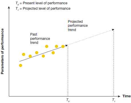
Actual sales results in a time series are plotted on the chart to identify the underlying trend. You will need to establish if that trend actually exists and whether it is consistent based on all past financial data. If you can successfully find the trend, your next task is to use it to predict the future.
That trend line is simply extended into the future to predict future sales. If a firm’s sale revenues have increased by 10% an average of every year in the past ten years, and there are not many changes in both internal business environment and external business environment, then, it might be expected that this trend will carry on in the foreseeable future.
The trend extrapolation technique is an important prediction tool for business managers, especially marketing managers, as it enables them to estimate sales data values beyond the original dataset.
How to extrapolate a trend?
Visually, the trend can be identified by a Line of Best Fit using simple linear regression with independent variable. Then, extrapolating simply means extending this line to make future prediction. Extrapolation simply takes the Line of Best Fit one move further in simple linear regression.
The chart below shows a trend of actual sales figures over a certain time period and an extrapolated trend:
So, how exactly can we extend the underlying trend into the future?
Method 1: Freehand sketching. Extrapolation is conducted by the manager who is plotting the future data and draws the ‘best’ fitting line by eye. This method, while neither perfect nor scientific, can give a first approximation of what the future sales results might look like.
Method 2: Moving averages. Extrapolation is done based on the use of moving averages which smooth out any variations in the dataset. Two four-point moving averages are averaged to come up with a centered trend. The final trend is then established by averaging out regular variations, and then extrapolated into the future using average seasonal variations, usually for each quarter.
Method 3: Regression line. Extrapolation is using the simple regression line for future predictions outside the range of past X values which were used to obtain the Line of Best Fit. Thos method works well when there is a clear correlation between two sets of numbers and there will be no changes to the status quo.
Method 4: Scenario writing. Extrapolation is using intuition and critical judgment about future sales to express probably future outcomes. Scenario writing focuses on future possibilities that the business is facing and how the business might act on these possible future situations.
Advantages of trend extrapolation
Trend extrapolation is very useful when predicting the near future. Also, this sales forecasting technique works well when there is a clear strong relationship between two sets of numbers such as spending on promotion and sales growth, or employee training and productivity improvement.
Disadvantages of trend extrapolation
Trend extrapolation assumes that sales patterns will not change at all in the future which is neither true nor very likely, especially when discussing long-term future. Hence, the predicted future sales levels might be completely inaccurate. Just think about how the Dotcom bubble in 2000, the global financial crisis of 2008 or the COVID-19 pandemic distorted business operations around the world in the last 15 years.
2. Fluctuations
Businesses and their managers heavily rely on past data behaviors in an attempt to predict the future.
Fluctuations show changes in past sales data caused by a certain reason. This information how sales varied in the past may indicate exactly how future sales will vary at similar point in time.
For example, a supermarket will experience very high demand for Christmas decorations in November and December while no demand in the remaining ten months of the year.
Different types of sales fluctuations
Let’s take a look now at different types of fluctuations regarding to sales of products:
- Cyclical fluctuations. These are caused by business cycles in an economy – mainly economic booms and economic recessions. Sales revenue will experience recurring fluctuations rising during the growth phase and falling during the decline phase. An example is when the demand for luxury products such as high-end cosmetics, expensive cars or holidays abroad increases during the economic growth in China as the country develops. Cyclical variations are tied to the business cycle in an economy and can last longer than one year.
- Seasonal fluctuations. These are period variations caused by the varying seasons in a year – mainly months or quarters of the year, or summers and winters. Sales revenue will fluctuate over a specified period of time. An example is when a retail business experiences an increase in demand and sales of winter clothing in cold winter and a decrease in demand and sales of the same winter clothes in warm summer. Seasonal variations are usually regular and repeated every year and occur within one year or less.
- Random fluctuations. These are unusual variations caused by a stand-out event – mainly natural and human-made crises such as public health epidemics, armed conflicts, natural disasters, corporate image crisis, etc. Sales revenue will be either unpredictably high or low caused by erratic and irregular factors that cannot be practically anticipated and prevented. An example is when there is a sudden increase in demand for air-conditioners during an extremely hot week during summertime. Random variations are unpredictable and can happen at any time anywhere in the world.
Most of variations in business management are seasonal variations as they are usually repeated and happen within one year.
3. Moving averages
A moving average is used to ‘smooth out’ the trend by removing any variations in the dataset produced by cyclical fluctuations, seasonal fluctuations and random fluctuations. In this way, an underlying trend can be identified and clear direction of that trend can be established.
Advantages of moving averages
The advantages of moving averages in sales forecasting include:
- More accurate method of identifying a trend and extrapolating that trend than simply using the arithmetic mean for predicting future sales levels based on current sales data.
- Useful for identifying seasonal variations for each time period (usually a quarter) and applying the knowledge to future predictions. Hence, moving averages aid sales planning in the foreseeable future.
- Helps with finding out various factors that might influence sales in the future. Once they have been identified, their impact on sales needs to be analyzed. Then, fairly accurate short-term sales forecasts can be made.
Disadvantages of moving averages
The disadvantages of moving averages in sales forecasting include:
- More complex to calculate especially for very large sales datasets than free-hand trend extrapolation.
- Not suitable for forecasting sales in the long-term. The longer the time period, the less accurate the projections become as they are entirely based on the past numbers.
- Factors in the internal business environment as well as external business environment can change unexpectedly any time.
Example of moving averages
In order to calculate moving averages, consider the data in the following table for a small business:
| [1] Year: | [2] Sales (USD$): |
|---|---|
| 2018 January | 300 |
| 2018 February | 300 |
| 2018 March | 400 |
| 2018 April | 500 |
| 2018 May | 400 |
| 2018 June | 300 |
There are a few ways to calculate moving averages. Three-point moving averages and four-point moving averages are the most common in sales forecasting.
A. Three-point moving average
Three-point moving average smooths out the trend, but not completely. Three-point moving averages are easier and quicker to calculate than four-point moving averages.
To calculate three-point moving average, average out three consecutive numbers in a time series – a number, the previous number and the next number – using arithmetic mean.
STEP 1: Start with calculating the arithmetic mean for the first three quarters in the time series including 2018 January, 2018 February and 2018 March:
(USD$300 + USD$300 + USD$400) / 3 = USD$333.33
STEP 2: Repeat this calculation for the next two items including 2018 Q3 and 2018 Q4:
(USD$300 + USD$400 + USD$500) / 3 = USD$400
(USD$400 + USD$500 + USD$400) / 3 = USD$433.33
STEP 3: Continue this process for the final item in the data set which is 2019 Q1:
(USD$500 + USD$400 + USD$300) / 3 = USD$400
This is how three-point moving averages can be presented in the table for better clarity:
| [1] Year: | [2] Sales (USD$): | [3] 3-Point Moving Average (USD$): |
|---|---|---|
| 2018 January | 300 | |
| 2018 February | 300 | 333.33 | (1+2+3) |
| 2018 March | 400 | 400 | (2+3+4) |
| 2018 April | 500 | 433.33 | (3+4+5) |
| 2018 May | 400 | 400 | (4+5+6) |
| 2018 June | 300 |
TIP: For any series of numbers you are able to calculate 2 less three-point moving averages than there are numbers in the series. It is because the first number does not have a previous number and the last number does not have a next number.
Three-point moving averages can be effectively used for working out the averages over a longer period of time as the average of three numbers (USD$333.33 (1+2+3)) can be compared with the actual sales (USD$300) for that period (2018 February).
Based on the above table, three-point moving show the underlying trend over the period of five months from 2018 February to 2018 May by smoothing out irregular fluctuations in that time series. With additional sales data after 2018 June, three-point moving averages could continue indefinitely.
B. Four-point moving average
Four-point moving average smooths out the trend more than three-point moving average. Four-point moving averages are harder and slower to calculate than three-point moving averages.
To calculate four-point moving average, average out four consecutive numbers in a time series using arithmetic mean.
STEP 1: Start with calculating the arithmetic mean for the first four quarters in the time series including 2018 Q1, 2018 Q2, 2018 Q3 and 2018 Q4:
(USD$1,000 + USD$1,200 + USD$900 + USD$1,100) / 4 = USD$1,050
STEP 2: Repeat this calculation for the next items including 2018 Q2, 2018 Q3, 2018 Q4 and 2019 Q1 as well as well as 2018 Q3, 2018 Q4, 2019 Q1 and 2019 Q2:
(USD$1,200 + USD$900 + USD$1,100 + USD$1,500) / 4 = USD$1,175
(USD$900 + USD$1,100 + USD$1,500 + USD$1,700) / 4 = USD$1,150
STEP 3: Continue this process for the final item in the data set which includes 2018 Q4, 2019 Q1, 2019 Q2 and 2019 Q3:
(USD$1,100 + USD$1,500 + USD$1,700 + USD$1,100) / 4 = USD$1,350
This is how four-point moving averages can be presented in the table for better clarity:
| [1] Year: | [2] Sales (USD$): | [3] 4-Point Moving Average (USD$): |
|---|---|---|
| 2018 Q1 | 1,000 | |
| 2018 Q2 | 1,200 | |
| 1,050 | (1+2+3+4) | ||
| 2018 Q3 | 900 | |
| 1,175 | (2+3+4+5) | ||
| 2018 Q4 | 1,100 | |
| 1,150 | (3+4+5+6) | ||
| 2019 Q1 | 1,500 | |
| 1,350 | (4+5+6+7) | ||
| 2019 Q2 | 1,700 | |
| 2019 Q3 | 1,100 |
TIP: For any series of numbers you are able to calculate 3 less four-point moving averages than there are numbers in the series.
Four-point moving averages can be effectively used for working out the averages when the data vary consistently over a longer period of time. For example, sales are higher in the second quarter of the year (Q2) but lower in the third quarter of the year (Q3). Because four-point moving averages fall on the mid-point (between the 2nd and 3rd number) which does not correspond with any actual sales figures, hence they need to be further adjusted using Centered TREND to make possible any comparisons with actual sales figures.
In addition to three-point moving average and four-point moving average, seven-point moving average can be used when daily sales figures are reported.
C. Trend forecasting using moving averages
When the data vary consistently over a longer period of time, four-point moving averages help to remove seasonal fluctuations from the dataset. The underlying trend can be established then by smoothing them out.
However, the resulting four-point moving averages figures do not fall on any particular quarter, but between two quarters. And, it is important for managers to compare the trend that falls on a particular quarter with actual sales values in that quarter. It is possible through the process called centering which is averaging two four-point moving averages.
TIP: The trend sales never equal the actual sales, hence could not be used to plan the future without further analysis. The trend on its own can only be used to show whether future sales are likely to be higher or lower than past sales.
The first Centered TREND [4] in the table below is found in the following way:
(USD$1,050 + USD$1,175) / 2 = USD$1,112.5
Moving averages can also be used to measure the values of variations from the trend. From this Centered TREND figure of USD$1,112.5 that falls on 2018 Q3, it is now possible to work out the specific seasonal variation in 2018 Q3.
USD$1,112.5 – USD$900 = -USD$212.5
The differences between the actual sales values and the Centered TRND are indeed seasonal fluctuations which are calculated in the following way:
Seasonal Variation [5] = Sales Revenue [2] – Centered TREND [4]
This can be presented in the table for better clarity:
| [1] Year: | [2] Sales (USD$): | [3] 4-Point Moving Average (USD$): | [4] Centered TREND (USD$): | [5] Seasonal Variation (USD$): |
|---|---|---|---|---|
| 2018 Q1 | 1,000 | |||
| 2018 Q2 | 1,200 | |||
| 1,050 | (1+2+3+4) | ||||
| 2018 Q3 | 900 | 1,112.5 | -212.5 | |
| 1,175 | (2+3+4+5) | ||||
| 2018 Q4 | 1,100 | 1,162.5 | -62.5 | |
| 1,150 | (3+4+5+6) | ||||
| 2019 Q1 | 1,500 | 1,250 | +250 | |
| 1,350 | (4+5+6+7) | ||||
| 2019 Q2 | 1,700 | |||
| 2019 Q3 | 1,100 |
TIP: Make sure you obtain the correct plus or minus sign for results of seasonal variations. If the result is negative, it means that in that the actual quarter sales are below the centered trend. If the result is positive, it means that the actual quarter sales are above the centered trend.
—
Forecasting a trend using the moving-average method is one of the biggest advantages of a time-series analysis.The trend line can be extended into the future to forecast future sales assuming that the trend from the past will continue in the similar way. To extrapolate the underlying trend using moving averages to forecast future actual sales per quarter, we need to recreate these quarterly variations around the extended trend.
STEP 1: Calculate four-quarter moving averages total [3].
STEP 2: Calculate eight-quarter moving averages total [4].
STEP 3: Work out the trend [5] by dividing eight-quarter moving averages total [4] by eight.
STEP 4: Calculate seasonal variations [6] as the difference between actual sales [2] and the trend [5]. The differences between the actual sales values and the Centered TREND are indeed seasonal fluctuations.
STEP 5: Find out the average seasonal variations for each of the four quarters: Q1, Q2, Q3, Q4. Average Seasonal Variations [7] smooth out the Actual Seasonal Variations [6]. Because these average variations are seasonal, they can be used to predict future sales by adjusting the extrapolated trend for each quarter in the future taking into account the recognized quarterly pattern of predictable variations from the past.
Average Seasonal Variation [7] for Q3 = Arithmetic mean of Seasonal Variations [6] in all Q3s
Average Seasonal Variation [7] for Q3 = (-USD$212.5 + (-USD$337.5) + USD$50) / 3 = -USD$166.67
| [1] Year: | [2] Sales (USD$): | [3] 4-Quarter Moving Total: | [4] 8-Quarter Moving Total: | [5] TREND: | [6] Seasonal Variation: | [7] Average Seasonal Variation: |
|---|---|---|---|---|---|---|
| 2018 Q1 | 1,000 | |||||
| 2018 Q2 | 1,200 | |||||
| 2018 Q3 | 900 | 1,112.5 | -212.5 | Q3: -166.67 | ||
| 2018 Q4 | 1,100 | 4,200 | 1,237.5 | -137.5 | Q4: -150 | |
| 2019 Q1 | 1,500 | 4,700 | 8,900 / 8 | 1,325 | 175 | Q1: 266.67 |
| 2019 Q2 | 1,700 | 5,200 | 9,900 / 8 | 1,375 | 325 | Q2: 54.17 |
| 2019 Q3 | 1,100 | 5,400 | 10,600 / 8 | 1,437.5 | -337.5 | Q3: -166.67 |
| 2019 Q4 | 1,300 | 5,600 | 11,000 / 8 | 1,387.5 | -87.5 | Q4: -150 |
| 2020 Q1 | 1,800 | 5,900 | 11,500 / 8 | 1,350 | 450 | Q1: 266.67 |
| 2020 Q2 | 1,000 | 5,200 | 11,100 / 8 | 1,412.5 | -412.5 | Q2: 54.17 |
| 2020 Q3 | 1,500 | 5,600 | 10,800 / 8 | 1,450 | 50 | Q3: -166.67 |
| 2020 Q4 | 1,400 | 5,700 | 11,300 / 8 | 1,625 | -225 | Q4: -150 |
| 2021 Q1 | 2,000 | 5,900 | 11,600 / 8 | 1,825 | 175 | Q1: 266.67 |
| 2021 Q2 | 2,200 | 7,100 | 13,000 / 8 | 1,950 | 250 | Q2: 54.17 |
| 2021 Q3 | 1,900 | 7,500 | 14,600 / 8 | |||
| 2021 Q4 | 2,000 | 8,100 | 15,600 / 8 |
While the actual sales figures [2] show an upward trend, there are also consistent seasonal patterns: sales in Quarter 1 and Quarter 2 are higher than the trend sales, and sales in Quarter 3 and Quarter 4 are lower than the trend sales. The results from the following table can be used for short-term sales forecasting.
STEP 6: Plot the actual sales revenue [2] on the chart. Add the trend [6] to the original time-series graph.
STEP 7: Read off the predicted sales revenue [2] for the future period 2022 Q1 which is USD$2,300.
STEP 8: Extrapolate the trend from the past into the future. The angle of the trend extension could be modified based on economic condition in the country.
STEP 9: Adjust this by the average seasonal variation [7] for Q1. How to do it? The trend forecast for 2022 Q1 will be the extrapolated trend for this quarter 2022 Q1. It is predicted sales revenue of USD$2,300 plus the average seasonal variation of Q1 which is USD$266.67. And that gives USD$2,566.67. In other words, both the trend line and the extrapolated trend smooth out seasonal variations.
It is important to remember that it is impossible to predict the exact sales levels in the future even with availability of robust past sales data. Additionally, some managers overestimate sales of their businesses to makes themselves look good among colleagues.
What is more, sales forecasting cannot be considered as science, but it rather helps business managers to identify any future opportunities and potential issues in regards to sales of products. And time-series analysis while being quite precise, it still remains as guestimation of the future.
